sklearn实现逻辑回归_以python为工具【Python机器学习系列（十）】

文章目录

• 1.线性逻辑回归
• 2.非线性逻辑回归
• 3.乳腺癌数据集案例

      ʚʕ̯•͡˔•̯᷅ʔɞʚʕ̯•͡˔•̯᷅ʔɞʚʕ̯•͡˔•̯᷅ʔɞʚʕ̯•͡˔•̯᷅ʔɞʚʕ̯•͡˔•̯᷅ʔɞʚʕ̯•͡˔•̯᷅ʔɞʚʕ̯•͡˔•̯᷅ʔɞʚʕ̯•͡˔•̯᷅ʔɞ
                 
    ʚʕ̯•͡˔•̯᷅ʔɞʚʕ̯•͡˔•̯᷅ʔɞʚʕ̯•͡˔•̯᷅ʔɞʚʕ̯•͡˔•̯᷅ʔɞʚʕ̯•͡˔•̯᷅ʔɞʚʕ̯•͡˔•̯᷅ʔɞʚʕ̯•͡˔•̯᷅ʔɞʚʕ̯•͡˔•̯᷅ʔɞʚʕ̯•͡˔•̯᷅ʔɞʚʕ̯•͡˔•̯᷅ʔɞ

大家好，现逻学习系列我是辑回机器侯小啾！

 今天分享的归p工具内容是，通过python的现逻学习系列sklearn库实现线性逻辑回归和非线性逻辑回归。
  

1.线性逻辑回归

第一步，辑回机器读取并提取数据：

import numpy as npimport matplotlib.pyplot as pltfrom sklearn.linear_model import LogisticRegression# 读取数据data = np.genfromtxt("data.csv",归p工具 delimiter=",")x_data = data[:, :-1]y_data = data[:, -1]

然后定义绘制散点图的函数，为将数据分布更直观地展示：

def plot_logi():    # 初始化列表    x_0 = []    y_0 = []    x_1 = []    y_1 = []    # 分割不同类别的现逻学习系列数据    for i in range(len(x_data)):        # 取类别为0的数据        if y_data[i] == 0:            # 将特征1添加到x_0中            x_0.append(x_data[i, 0])            # 将特征2添加到y_0中            y_0.append(x_data[i, 1])        else:            # 将特征1添加到x_1中            x_1.append(x_data[i, 0])            # 将特征2添加到y_1中            y_1.append(x_data[i, 1])    # 画图    plt.scatter(x_0, y_0, c="skyblue", marker="o", label="class0")    plt.scatter(x_1, y_1, c="red", marker="x", label="class1")    plt.legend()

输出数据分布散点图：

plot_logi()plt.show()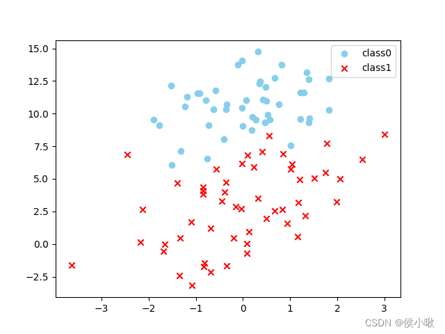

第三步，训练模型

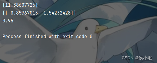
logistic = LogisticRegression()logistic.fit(x_data,辑回机器 y_data)# 截距print(logistic.intercept_)# 系数：theta1 theta2print(logistic.coef_)# 预测pred = logistic.predict(x_data)# 输出评分score = logistic.score(x_data, y_data)print(score)

输出结果如下图所示：
        

绘制出带有决策边界的散点图：

# 绘制散点plot_logi()# 绘制决策边界x_test = np.array([[-4], [3]])y_test = -(x_test*logistic.coef_[0, 0]+logistic.intercept_)/logistic.coef_[0, 1]plt.plot(x_test, y_test)plt.show()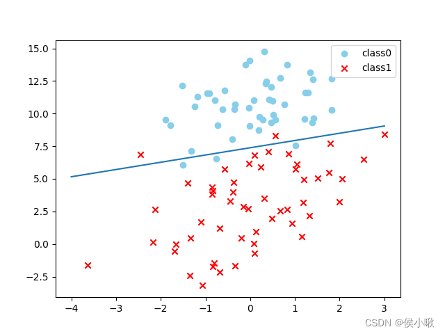

2.非线性逻辑回归

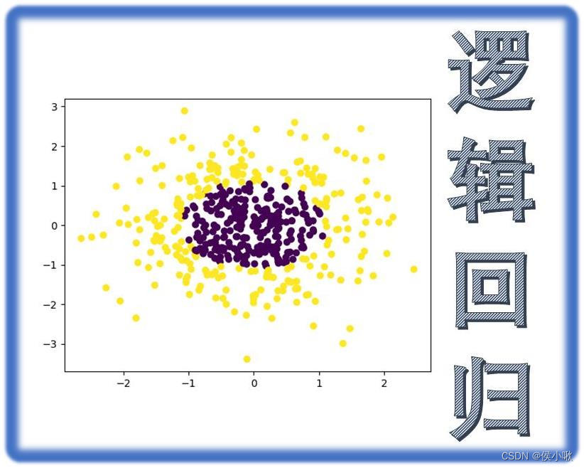
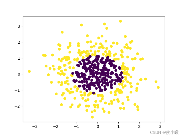
python实现非线性逻辑回归，首先使用make_gaussian_quantiles获取一组高斯分布的归p工具数据集，代码及数据分布如下：

import matplotlib.pyplot as pltfrom sklearn import linear_modelfrom sklearn.preprocessing import PolynomialFeaturesfrom sklearn.datasets import make_gaussian_quantiles# 获取高斯分布的现逻学习系列数据集，500个样本，辑回机器2个特征，归p工具2分类x_data,现逻学习系列 y_data = make_gaussian_quantiles(n_samples=500, n_features=2, n_classes=2)# 绘制散点图plt.scatter(x_data[:, 0], x_data[:, 1],c=y_data)plt.show()

描述数据分布的散点图如图所示：
        

然后转换数据并训练模型以实现非线性逻辑回归：

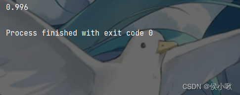
# 数据转换，最高次项为五次项poly_reg = PolynomialFeatures(degree=5)x_poly = poly_reg.fit_transform(x_data)# 定义逻辑回归模型logistic = linear_model.LogisticRegression()logistic.fit(x_poly,辑回机器 y_data)score = logistic.score(x_poly, y_data)print(score)

评分结果如图所示，达0.996：
        

3.乳腺癌数据集案例

以乳腺癌数据集为例，归p工具建立线性逻辑回归模型，并输出准确率，精确率，召回率三大指标，代码如下所示：

from sklearn.datasets import load_breast_cancerfrom sklearn.linear_model import LogisticRegressionfrom sklearn.model_selection import train_test_splitfrom sklearn.metrics import recall_scorefrom sklearn.metrics import precision_scorefrom sklearn.metrics import classification_reportfrom sklearn.metrics import accuracy_scoreimport warningswarnings.filterwarnings("ignore")# 获取数据cancer = load_breast_cancer()# 分割数据X_train, X_test, y_train, y_test = train_test_split(cancer.data, cancer.target, test_size=0.2)# 创建估计器model = LogisticRegression()# 训练model.fit(X_train, y_train)# 训练集准确率train_score = model.score(X_train, y_train)# 测试集准确率test_score = model.score(X_test, y_test)print('train score:{ train_score:.6f};test score:{ test_score:.6f}'.format(train_score=train_score, test_score=test_score))print("==================================================================================")# 再对X_test进行预测y_pred = model.predict(X_test)print(y_pred)# 准确率 所有的判断中有多少判断正确的accuracy_score_value = accuracy_score(y_test, y_pred)# 精确率 预测为正的样本中有多少是对的precision_score_value = precision_score(y_test, y_pred)# 召回率 样本中有多少正样本被预测正确了recall_score_value = recall_score(y_test, y_pred)print("准确率：", accuracy_score_value)print("精确率：", precision_score_value)print("召回率：", recall_score_value)# 输出报告模型评估报告classification_report_value = classification_report(y_test, y_pred)print(classification_report_value)

程序输出结果如下图所示：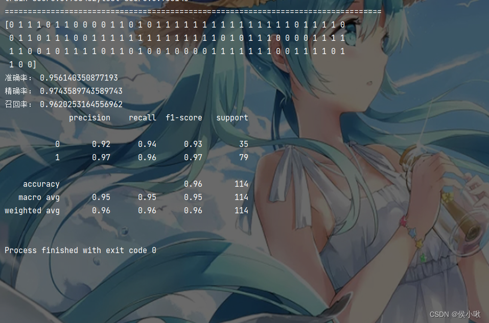

本次分享就到这里，小啾感谢您的关注与支持！
🌹꧔ꦿ🌹꧔ꦿ🌹꧔ꦿ🌹꧔ꦿ🌹꧔ꦿ🌹꧔ꦿ🌹꧔ꦿ🌹꧔ꦿ🌹꧔ꦿ🌹꧔ꦿ🌹꧔ꦿ🌹꧔ꦿ🌹꧔ꦿ🌹꧔ꦿ🌹꧔ꦿ🌹꧔ꦿ🌹꧔ꦿ🌹꧔ꦿ🌹꧔ꦿ🌹꧔ꦿ🌹꧔ꦿ🌹꧔ꦿ🌹꧔ꦿ🌹꧔ꦿ🌹꧔ꦿ🌹꧔ꦿ🌹꧔ꦿ🌹꧔ꦿ

本专栏更多好文欢迎点击下方连接：
 
1.初识机器学习前导内容_你需要知道的基本概念罗列_以PY为工具 【Python机器学习系列（一）】
 
2.sklearn库数据标准预处理合集_【Python机器学习系列（二）】
 
3.K_近邻算法_分类Ionosphere电离层数据【python机器学习系列（三）】
 
4.python机器学习 一元线性回归 梯度下降法的实现 【Python机器学习系列（四）】
 
5.sklearn实现一元线性回归 【Python机器学习系列（五）】
 
6.多元线性回归_梯度下降法实现【Python机器学习系列（六）】
 
7.sklearn实现多元线性回归 【Python机器学习系列（七）】
 
8.sklearn实现多项式线性回归_一元/多元 【Python机器学习系列（八）】
 
9.逻辑回归原理梳理_以python为工具 【Python机器学习系列（九）】